Mathematics and transforms are essential as they help us define how objects and light interact in a 3D scene. Coordinate systems and vectors are used to position objects and describe directions. Transforms like moving, rotating, or scaling objects align them in the scene. Rays, which represent paths of light, are traced to find where they hit objects, while bounding boxes make these calculations faster by narrowing down what needs to be checked. These tools work together to simulate real-world lighting and materials accurately and efficiently.
Coordinate Systems
A coordinate system is a method for uniquely determining the position of points in a space.
They are fundamental for representing positions in space, and their handedness (left vs. right) has significant implications.
Understanding handedness is essential for ensuring consistent behavior in simulations, animations, and any application involving spatial calculations.
The most common coordinate systems are:
- Cartesian coordinates: defined by orthogonal axes (X, Y, Z).
- Polar coordinates: defined by a distance from a reference point and an angle.
- Spherical coordinates: defined by a distance from a reference point and two angles.
Handedness (Left vs Right)
Handedness refers to the orientation of the coordinate system in three-dimensional space. It helps in determining the relative position and rotation of objects within that space. There are two primary types of handedness:
1. Right-Handed Coordinate System (RHS) 2. Left-Handed Coordinate System (LHS)
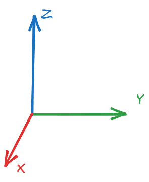
Right-Handed Coordinate System (RHS)
In a right-handed coordinate system:
• Imagine you are holding the three axes of the coordinate system with your right hand.
• Your thumb points in the direction of the positive Z-axis, your index finger points in the direction of the positive X-axis, and your middle finger points in the direction of the positive Y-axis.
This arrangement can be visualized as follows:
Right-Handed Coordinate System (RHS).
In this system, if you curl your fingers from the X-axis toward the Y-axis, your thumb points in the direction of the Z-axis.
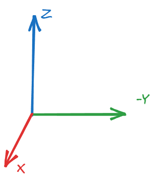
Left-Handed Coordinate System (LHS)
In a left-handed coordinate system:
• You hold the axes with your left hand instead.
• Your thumb points in the direction of the positive Z-axis, your index finger points in the direction of the positive X-axis, and your middle finger points in the direction of the negative Y-axis.
This arrangement looks like this:
Left-Handed Coordinate System (LHS).
In this case, curling your fingers from the X-axis toward the Y-axis points your thumb in the direction of the negative Z-axis.
Importance of Handedness
1. Consistency in Graphics and Physics: Handedness is critical in 3D graphics and physics simulations. A right-handed system is commonly used in most computer graphics applications (e.g., OpenGL), while a left-handed system might be used in others (e.g., Direct3D).
2. Vector Operations: Operations such as the cross product can yield different results based on the handedness of the coordinate system, affecting object orientation and transformations.
3. Geometric Interpretations: Handedness can affect how shapes are drawn and manipulated in a 3D space. If you switch from one handedness to another, the interpretation of the angles, rotations, and object orientations may change.
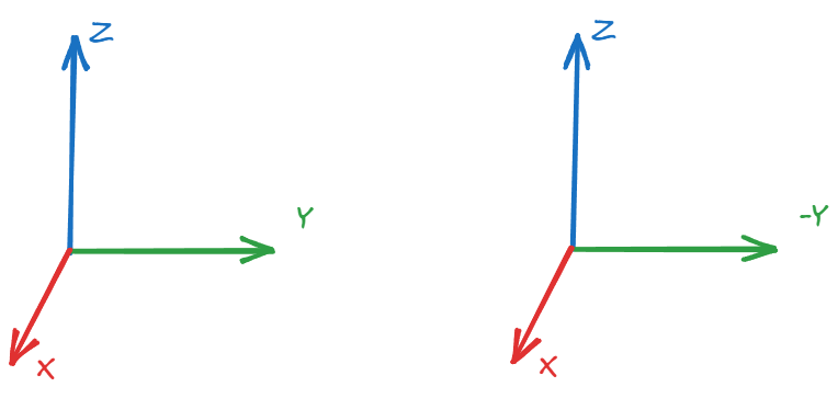
Comparing Coordinate System.
Mathematical Representation of Handedness
Let's look at how the right-hand and left-hand systems can be mathematically represented. Suppose you have two vectors \( \mathbf{a} \) and \( \mathbf{b} \) in 3D space.
In a right-handed system, the cross product \( \mathbf{c} = \mathbf{a} \times \mathbf{b} \) gives a vector \( \mathbf{c} \) that points in the positive Z direction.
In a left-handed system, the same cross product yields a vector \( \mathbf{c} \) that points in the negative Z direction.
Let's write a JavaScript function that calculates the cross product of two vectors, and we can observe how the handedness affects the result.
function crossProduct(a, b) {
    return [
        a[1] * b[2] - a[2] * b[1], // X component
        a[2] * b[0] - a[0] * b[2], // Y component
        a[0] * b[1] - a[1] * b[0]  // Z component
    ];
}

// Example vectors for right-handed system
const vectorA = [1, 0, 0]; // X-axis
const vectorB = [0, 1, 0]; // Y-axis

const rightHandedCrossProduct = crossProduct(vectorA, vectorB);
console.log("Cross Product (Right-Handed):", rightHandedCrossProduct); // Output: [0, 0, 1]

// Example vectors for left-handed system (manually flipping the Z-axis)
const leftHandedCrossProduct = crossProduct(vectorA, [-0, -1, 0]); // flipping Y to negative
console.log("Cross Product (Left-Handed):", leftHandedCrossProduct); // Output: [0, 0, -1]
Vectors
A vector is a mathematical object that has both magnitude (length) and direction. Vectors are often represented in a Cartesian coordinate system with components, e.g., a 3D vector can be represented as \( \mathbf{v} = (x, y, z) \).
Dot Product
The dot product of two vectors \( \mathbf{a} = (a_x, a_y, a_z) \) and \( \mathbf{b} = (b_x, b_y, b_z) \) is calculated as:
The cross product of two vectors \( \mathbf{a} \) and \( \mathbf{b} \) results in a vector that is perpendicular to both \( \mathbf{a} \) and \( \mathbf{b} \). It is calculated as:
Normalization of a vector involves scaling the vector so that it has a magnitude of 1, which is known as a unit vector. The formula for normalizing a vector \( \mathbf{v} = (v_x, v_y, v_z) \) is:
We often need to construct a local coordinate system when provided with a single 3D vector. Using the cross product of two vectors, we can create a set of three orthogonal vectors that define a local coordinate system. Since the cross product between two vectors is perpendicular to both, applying the cross product twice yields three orthogonal vectors. However, the second and third vectors are unique only up to a rotation around the given vector.
Steps to Construct the Coordinate System
1. Start with a normalized vector \( \mathbf{v_1} \).
The given vector \( \mathbf{v_1} \) is assumed to be normalized, meaning \( \mathbf{v_1} \cdot \mathbf{v_1} = 1 \).
2. Generate a second vector \( \mathbf{v_2} \) that is perpendicular to \( \mathbf{v_1} \).
One simple way to do this is by zeroing one component of \( \mathbf{v_1} \), swapping the remaining two, and negating one of them.
3. Cross product of \( \mathbf{v_1} \) and \( \mathbf{v_2} \) to get a third vector \( \mathbf{v_3} \) that is perpendicular to both.
The resulting vector \( \mathbf{v_3} \) will complete the orthogonal set of vectors.
Example of Vector Construction
Let \( \mathbf{v_1} = (x, y, z) \) be the normalized input vector.
1. Construct a Perpendicular Vector \( \mathbf{v_2} \):
If \( x \) is non-zero, we can choose \( \mathbf{v_2} = (-y, x, 0) \).
This ensures that \( \mathbf{v_1} \cdot \mathbf{v_2} = 0 \), meaning the two vectors are perpendicular.
2. Calculate the Third Vector \( \mathbf{v_3} \):
Use the cross product:
\[
\mathbf{v_3} = \mathbf{v_1} \times \mathbf{v_2}
\]
We chose the first non-zero - however, you could also modify the algorithm to search for the largest component instead (better numerical).
JavaScript Example
Here's a simple JavaScript implementation that constructs an orthogonal coordinate system from a given normalized vector:
function crossProduct(v1, v2) {
    return [
        v1[1] * v2[2] - v1[2] * v2[1],
        v1[2] * v2[0] - v1[0] * v2[2],
        v1[0] * v2[1] - v1[1] * v2[0]
    ];
}

function normalize(v) {
    const length = Math.sqrt(v[0]**2 + v[1]**2 + v[2]**2);
    return [v[0] / length, v[1] / length, v[2] / length];
}

function constructCoordinateSystem(v1) {
    // Assume v1 is already normalized
    let v2;

    // Choose a simple perpendicular vector
    if (Math.abs(v1[0]) > 0.001) {
        v2 = [-v1[1], v1[0], 0]; // swap y and x, and negate one
    } else {
        v2 = [0, -v1[2], v1[1]]; // swap z and y, and negate one
    }

    // Normalize v2
    v2 = normalize(v2);

    // Compute v3 as the cross product of v1 and v2
    const v3 = crossProduct(v1, v2);

    return {
        v1: v1,
        v2: v2,
        v3: v3
    };
}

// Example Usage
const v1 = normalize([1, 2, 3]); // Input vector (normalized)
const coordinateSystem = constructCoordinateSystem(v1);

console.log("v1:", coordinateSystem.v1);
console.log("v2:", coordinateSystem.v2);
console.log("v3:", coordinateSystem.v3);
Points
A point is defined as a specific location in space, characterized by its coordinates in a given coordinate system. For instance, in a 2D Cartesian coordinate system, a point can be represented as \( P(x, y) \), indicating its position along the X and Y axes. Similarly, in a 3D space, a point is represented as \( P(x, y, z) \), indicating its location along the X, Y, and Z axes. Points are static entities; they do not possess direction or magnitude, but rather, they denote a precise location in space.
Differences Between Points and Vectors
The primary difference between points and vectors lies in their characteristics and operations:
1. Representation:
A point is represented solely by its coordinates, while a vector is represented by its components and includes a direction.
2. Nature:
A point is a static location, whereas a vector is a dynamic entity that describes a direction and magnitude.
3. Operations:
Points can be manipulated using vector operations, such as addition and subtraction. For example, if you have a point \( P_1(x_1, y_1) \) and a vector \( \mathbf{v}(dx, dy) \), you can find a new point \( P_2 \) by adding the vector to the point:
\[
P_2 = P_1 + \mathbf{v} = (x_1 + dx, y_1 + dy).
\]
This operation effectively "moves" the point in the direction specified by the vector.
Common Operations
1. Translation: As mentioned above, translating a point involves adding a vector to the point's coordinates. This operation shifts the point to a new location.
2. Distance Calculation: The distance between two points can be calculated using the Euclidean distance formula. For points \( P_1(x_1, y_1) \) and \( P_2(x_2, y_2) \) in 2D space, the distance \( d \) is given by:
\[
d = \sqrt{(x_2 - x_1)^2 + (y_2 - y_1)^2}.
\]
In 3D space, the formula extends to:
\[
d = \sqrt{(x_2 - x_1)^2 + (y_2 - y_1)^2 + (z_2 - z_1)^2}.
\]
Normals
A normal vector is perpendicular to a surface at a given point and plays a crucial role in lighting calculations, surface shading, and collision detection.
How Normals Are Computed
Normals can be calculated for various geometrical primitives:
1. Flat Surfaces: For a flat polygon (like a triangle), the normal can be computed using the cross product of two of its edges. For a triangle defined by three points \( P_1, P_2, P_3 \):
The normal \( \mathbf{N} \) is computed as:
\[
\mathbf{N} = \mathbf{v_1} \times \mathbf{v_2}
\]
Normalize \( \mathbf{N} \) to ensure it has a unit length.
2. Smooth Surfaces: For a smooth surface, normals can be averaged from the normals of the surrounding polygons that share a vertex. This helps create a smoother appearance on curved surfaces.
Example: Calculating Normals in JavaScript
Here's an example of how to compute the normal vector for a triangle defined by three vertices in JavaScript:
// Function to calculate the normal of a triangle
function calculateNormal(p1, p2, p3) {
    // Create vectors v1 and v2
    const v1 = [p2[0] - p1[0], p2[1] - p1[1], p2[2] - p1[2]]; // Vector from p1 to p2
    const v2 = [p3[0] - p1[0], p3[1] - p1[1], p3[2] - p1[2]]; // Vector from p1 to p3

    // Calculate the cross product to find the normal
    const normal = [
        v1[1] * v2[2] - v1[2] * v2[1], // x component
        v1[2] * v2[0] - v1[0] * v2[2], // y component
        v1[0] * v2[1] - v1[1] * v2[0]  // z component
    ];

    // Normalize the normal vector
    const length = Math.sqrt(normal[0] ** 2 + normal[1] ** 2 + normal[2] ** 2);
    return [normal[0] / length, normal[1] / length, normal[2] / length]; // Return normalized normal
}

// Example usage
const p1 = [0, 0, 0];
const p2 = [1, 0, 0];
const p3 = [0, 1, 0];

const normal = calculateNormal(p1, p2, p3);
console.log("Normal Vector:", normal); // Output: [0, 0, 1] (Normal points in the positive Z direction)
Rays
Rays are fundamental to rendering techniques such as ray tracing, where they are used to simulate the interaction of light with surfaces to produce realistic images. A ray is typically defined by its origin point and a direction vector, allowing it to describe a path in three-dimensional space. Mathematically, a ray can be represented as:
\[
\mathbf{R}(t) = \mathbf{O} + t \cdot \mathbf{D}
\]
where:
\( \mathbf{R}(t) \) is the point along the ray at parameter \( t \),
\( \mathbf{O} \) is the ray's origin,
\( \mathbf{D} \) is the direction vector,
\( t \) is a scalar that determines how far along the ray we are.
Rays are instrumental in various rendering processes, including shadow calculations, reflection, and refraction, making them crucial for achieving photorealistic imagery.
Ray Differentials
Ray differentials enhance the basic ray concept by considering variations in rays that are closely associated with a primary ray. In rendering scenarios, particularly when dealing with anti-aliasing and depth of field, understanding how rays deviate from their original paths is essential for producing high-quality images.
Ray differentials help quantify how a primary ray, originating from a pixel on the image plane, can be perturbed to create additional rays that sample the scene more effectively. These variations are especially important in scenarios where light interacts with complex geometries, as they can significantly improve image quality by reducing artifacts such as jagged edges and blurry backgrounds.
Importance of Ray Differentials
1. Anti-Aliasing: By generating multiple rays for a single pixel, ray differentials enable better sampling of a scene, allowing for smoother edges and reducing visual artifacts. This is particularly useful in scenes with high-frequency details.
2. Depth of Field: In realistic rendering, depth of field effects blur objects that are out of focus. Ray differentials allow for simulating the various positions from which light can enter a lens, thereby producing more natural transitions between sharp and blurred areas.
3. Global Illumination: Ray differentials contribute to more accurate global illumination calculations by allowing for a more comprehensive sampling of light interactions within a scene, improving realism in lighting.
Calculating Ray Differentials
Ray differentials can be calculated by perturbing the origin of the primary ray and its direction. For instance, if \( \mathbf{R}_0 \) is the primary ray, you can generate ray differentials \( \mathbf{R}_{x} \) and \( \mathbf{R}_{y} \) to sample neighboring rays around the pixel:
Here, \( \delta_x \) and \( \delta_y \) are small perturbations, and \( \mathbf{D}_{u} \) and \( \mathbf{D}_{v} \) are direction vectors along the image plane.
Here, \( \epsilon_x \) and \( \epsilon_y \) are small perturbations that adjust the ray's direction slightly.
Example: Implementing Ray Differentials in JavaScript
Here is an example that demonstrates how to compute ray differentials in a JavaScript context:
class Ray {
    constructor(origin, direction) {
        this.origin = origin; // [x, y, z]
        this.direction = direction; // [dx, dy, dz]
    }

    // Method to create ray differentials
    createDifferentials(deltaX, deltaY) {
        // Define small perturbations for origin and direction
        const perturbationX = [deltaX, 0, 0]; // X perturbation
        const perturbationY = [0, deltaY, 0]; // Y perturbation

        const rayX = new Ray(
            [this.origin[0] + perturbationX[0], this.origin[1] + perturbationX[1], this.origin[2] + perturbationX[2]],
            this.direction
        );

        const rayY = new Ray(
            [this.origin[0] + perturbationY[0], this.origin[1] + perturbationY[1], this.origin[2] + perturbationY[2]],
            this.direction
        );

        return { rayX, rayY };
    }
}

// Example usage
const primaryRay = new Ray([0, 0, 0], [0, 0, -1]);
const { rayX, rayY } = primaryRay.createDifferentials(0.01, 0.01);

console.log("Primary Ray:", primaryRay);
console.log("Ray Differential X:", rayX);
console.log("Ray Differential Y:", rayY);
Bounding Boxes
Bounding boxes are essential geometric structures used to simplify collision detection, visibility testing, and spatial partitioning. They enclose a geometric shape or object in a defined volume, providing a quick way to check for intersections or proximity without needing to consider the object's detailed geometry.
Why Bounding Boxes?
Bounding boxes serve several crucial purposes:
1. Collision Detection: They simplify the process of checking for collisions between complex objects. If the bounding boxes of two objects do not intersect, it can be inferred that the objects themselves do not intersect.
2. Efficiency: Calculating intersections between bounding boxes is computationally cheaper than testing intersections between complex shapes. This efficiency is vital in real-time applications, such as video games.
3. Culling: In rendering, bounding boxes can help determine whether objects are within the view frustum. If a bounding box is outside the frustum, the object can be culled (not rendered), improving performance.
4. Spatial Partitioning: Bounding boxes can be used to organize and index objects in a scene, facilitating more efficient rendering and collision detection through structures like quad-trees or BSP trees.
Axis-Aligned Bounding Boxes (AABBs)
Axis-aligned bounding boxes (AABBs) are bounding boxes whose faces are aligned with the coordinate axes. An AABB is defined by two opposite corners, usually represented as the minimum and maximum points:
\[
\text{AABB} = [\text{min}(x, y, z), \text{max}(x, y, z)]
\]
Characteristics of AABBs
- Simplicity: AABBs are easy to calculate and manipulate, as they only require the minimum and maximum coordinates of the enclosed geometry.
- Fast Intersection Tests: Checking if two AABBs intersect is straightforward and efficient, requiring only comparisons of the min and max coordinates along each axis.
Example: Implementing AABBs in JavaScript
Here's a basic implementation of an AABB in JavaScript, including a method to check for intersection:
Oriented bounding boxes (OBBs) are bounding boxes that can rotate and align with the object's orientation, providing a tighter fit around complex shapes than AABBs. An OBB is defined by a center point, an orientation (usually represented by a rotation matrix), and half-extents along each axis.
Characteristics of OBBs
- Better Fit: OBBs can conform more closely to the shape of the object, reducing empty space and improving collision detection accuracy.
- Complex Intersection Tests: Checking for intersection between OBBs is more complex than AABBs, often requiring computational geometry techniques like the Separating Axis Theorem (SAT).
Example: Implementing OBBs in JavaScript
Here's a basic implementation of an OBB in JavaScript, including a method to check for intersection using the Separating Axis Theorem:
class OBB {
    constructor(center, halfExtents, rotationMatrix) {
        this.center = center; // [xCenter, yCenter, zCenter]
        this.halfExtents = halfExtents; // [halfX, halfY, halfZ]
        this.rotationMatrix = rotationMatrix; // 3x3 rotation matrix
    }

    // Method to check intersection with another OBB using the Separating Axis Theorem (SAT)
    intersects(other) {
        // Transform the center of the other OBB to the local space of this OBB
        const toOtherCenter = [
            other.center[0] - this.center[0],
            other.center[1] - this.center[1],
            other.center[2] - this.center[2]
        ];

        // Project the half extents of both OBBs onto the axes
        const axes = this.getAxes();
        for (const axis of axes) {
            const [projection1, projection2] = this.projectOntoAxis(axis, other, toOtherCenter);
            if (this.overlap(projection1, projection2) === 0) {
                return false; // No overlap, OBBs do not intersect
            }
        }
        return true; // OBBs intersect
    }

    // Helper methods (getAxes, projectOntoAxis, overlap) would need to be implemented for full functionality
}

// Example usage
const obb1 = new OBB([0, 0, 0], [1, 1, 1], /* rotation matrix */);
const obb2 = new OBB([0.5, 0.5, 0.5], [1, 1, 1], /* rotation matrix */);
const obb3 = new OBB([3, 3, 3], [1, 1, 1], /* rotation matrix */);

console.log("OBB1 intersects OBB2:", obb1.intersects(obb2)); // Depends on actual implementation
console.log("OBB1 intersects OBB3:", obb1.intersects(obb3)); // Depends on actual implementation
Transformations
Transformations are essential for efficiently and clearly manipulating data. They include operations such as translation, scaling, and rotation. To perform these transformations efficiently and consistently, homogeneous coordinates are used, which facilitate linear transformations in projective geometry.
Homogeneous Coordinates
Homogeneous coordinates extend traditional Cartesian coordinates by adding an extra coordinate, \(w\). For a point \((x, y, z)\) in 3D space, the homogeneous coordinates are represented as \((x, y, z, w)\). The conversion from Cartesian to homogeneous coordinates is given by:
\[
(x, y, z) \rightarrow (x, y, z, 1)
\]
When \(w \neq 0\), the original coordinates can be retrieved by dividing by \(w\):
The use of homogeneous coordinates allows transformations to be represented as matrix multiplications, which can simplify the computation of multiple transformations (e.g., rotation followed by translation).
Example: The homogeneous coordinates for the point \((2, 3, 4)\) would be \((2, 3, 4, 1)\).
Identity Transformation
The identity transformation is a transformation that leaves objects unchanged. In matrix form, the identity matrix \(I\) for 3D transformations is:
Translation moves an object in space by adding a vector \((tx, ty, tz)\) to each of its coordinates. The translation matrix \(T\) for 3D transformations is:
function scale(point, sx, sy, sz) {
    const S = [
        [sx, 0, 0, 0],
        [0, sy, 0, 0],
        [0, 0, sz, 0],
        [0, 0, 0, 1]
    ];

    const v = [point[0], point[1], point[2], 1];

    const result = [];
    for (let i = 0; i < 4; i++) {
        result[i] = 0;
        for (let j = 0; j < 4; j++) {
            result[i] += S[i][j] * v[j];
        }
    }

    return result.slice(0, 3); // return (x, y, z)
}

// Example usage
const scaledPoint = scale([2, 3, 4], 2, 3, 4);
console.log(scaledPoint); // Output: [4, 9, 16]
Euler Rotations
Euler rotations are a method of representing 3D rotations using three angles, typically around the x, y, and z axes. The rotation matrices for each axis are:
To rotate around an arbitrary axis defined by a unit vector \(\mathbf{u} = (u_x, u_y, u_z)\) by an angle \(\theta\), we can use the Rodrigues' rotation formula. The rotation matrix \(R\) is given by:
\[
R = I + \sin(\theta) K + (1 - \cos(\theta)) K^2
\]
where \(K\) is the skew-symmetric matrix of \(\mathbf{u}\):
The look-at transformation creates a viewing matrix that positions the camera at a specific point in 3D space and directs it towards a target point. The transformation typically requires the following inputs:
Transformations are essential for manipulating points, vectors, normals, rays, and bounding boxes. Using homogeneous coordinates and matrix multiplication, complex sequences of transformations like translation, scaling, and rotation can be applied efficiently. In this section, we will cover how transformations are applied to different entities, their mathematical representations, and code implementations in JavaScript.
Points
When applying a transformation to a point, we typically work with homogeneous coordinates \((x, y, z, 1)\). This allows us to use a 4x4 transformation matrix to perform operations like translation and scaling.
Mathematical Representation
Given a point \(P = (x, y, z, 1)\) and a transformation matrix \(T\), the transformed point \(P'\) is calculated as:
\[
P' = T \cdot P
\]
Example: Translation
Translating the point \(P = (2, 3, 4)\) by \(t_x = 1\), \(t_y = 1\), and \(t_z = 1\):
function applyTransformationToPoint(point, matrix) {
    const [x, y, z] = point;
    const v = [x, y, z, 1]; // Convert point to homogeneous coordinates

    const transformed = [];
    for (let i = 0; i < 4; i++) {
        transformed[i] = 0;
        for (let j = 0; j < 4; j++) {
            transformed[i] += matrix[i][j] * v[j];
        }
    }

    return transformed.slice(0, 3); // return (x', y', z')
}

// Example: Translation matrix
const translationMatrix = [
    [1, 0, 0, 1],
    [0, 1, 0, 1],
    [0, 0, 1, 1],
    [0, 0, 0, 1]
];

const point = [2, 3, 4];
const translatedPoint = applyTransformationToPoint(point, translationMatrix);
console.log(translatedPoint); // Output: [3, 4, 5]
Vectors
Unlike points, when applying transformations to vectors, we ignore the translation component of the matrix (i.e., the last column). For scaling and rotation, we apply the same matrix as with points, except the vector's homogeneous coordinate is \((x, y, z, 0)\).
Mathematical Representation
Given a vector \(V = (x, y, z, 0)\) and a transformation matrix \(T\), the transformed vector \(V'\) is calculated as:
\[
V' = T \cdot V
\]
Example: Scaling
Scaling a vector \(V = (1, 2, 3)\) by factors of \(2\) along all axes:
Transforming normals is different from transforming vectors because scaling and shearing can distort the direction of the normal. To correctly transform a normal, we use the inverse transpose of the transformation matrix.
Mathematical Representation
Given a normal \(N = (x, y, z, 0)\) and a transformation matrix \(T\), the transformed normal \(N'\) is calculated using the inverse transpose of \(T\):
Then we transpose this matrix and apply it to the normal.
JavaScript Code
function applyTransformationToNormal(normal, matrix) {
    const inverseMatrix = inverse(matrix);
    const transposeMatrix = transpose(inverseMatrix);
    return applyTransformationToVector(normal, transposeMatrix);
}

// Helper functions: Matrix inverse and transpose (assuming 4x4 matrices)
function inverse(matrix) {
    // Compute the inverse of the 4x4 matrix (implementation depends on the library)
    ....

}

function transpose(matrix) {
    const result = [];
    for (let i = 0; i < 4; i++) {
        result[i] = [];
        for (let j = 0; j < 4; j++) {
            result[i][j] = matrix[j][i];
        }
    }
    return result;
}
Rays
To apply a transformation to a ray, both the origin and the direction must be transformed independently. The origin is treated as a point \((x, y, z, 1)\), and the direction is treated as a vector \((x, y, z, 0)\).
Mathematical Representation
Given a ray \(R = (O, D)\) where \(O\) is the origin and \(D\) is the direction, the transformed ray \(R'\) is:
\[
O' = T \cdot O, \quad D' = T \cdot D
\]
Example
Apply a translation to a ray with origin \((0, 0, 0)\) and direction \((1, 0, 0)\):
Discuss applying a transformation to an AABB. We apply a transform to an AABB by transforming all of its corners and compute a new AABB that bounds the transformed points.
Example: Transform an AABB
For an AABB defined by its minimum and maximum corners \((x_{min}, y_{min}, z_{min})\) and \((x_{max}, y_{max}, z_{max})\), transform all 8 corners using the transformation matrix.
Transformations can be combined by multiplying their corresponding matrices. This allows multiple transformations to be applied in sequence. For example, combining translation, scaling, and rotation can be done by multiplying the matrices for each transformation.
Mathematical Representation
Given transformations \(T_1, T_2, \ldots, T_n\), the final transformation \(T\) is:
\[
T = T_n \cdot \ldots \cdot T_2 \cdot T_1
\]
Example: Combining Translation and Rotation
Combine translation by \((1, 1, 1)\) and rotation around the z-axis by \(90^\circ\):
\[
T = R_z(90^\circ) \cdot T_{translate}
\]
JavaScript Code
function multiplyMatrices(A, B) {
    const result = [];
    for (let i = 0; i < 4; i++) {
        result[i] = [];
        for (let j = 0; j < 4; j++) {
            result[i][j] = 0;
            for (let k = 0; k < 4; k++) {
                result[i][j] += A[i][k] * B[k][j];
            }
        }
    }
    return result;
}

const combinedMatrix = multiplyMatrices(rotationMatrixZ, translationMatrix);
Transformations and Coordinate System Handedness
When applying transformations, the choice of handedness can affect how rotations and cross-products behave.
• Right-handed systems: Positive rotations follow the right-hand rule.
• Left-handed systems: Positive rotations follow the left-hand rule.
When switching between handedness, the sign of the z-coordinate (or y-coordinate depending on the system) must be inverted.
JavaScript Code
To switch between coordinate systems:
function switchHandedness(point) {
    return [point[0], point[1], -point[2]]; // Switch from right-handed to left-handed by inverting z-axis
}
Animating Transformations
Animations are often achieved by smoothly transitioning between different transformations. This involves methods like quaternion interpolation for smooth rotations and managing transformations applied to objects like bounding boxes. In this section, we will cover quaternions, quaternion interpolation, and animating bounding boxes in detail, with equations and JavaScript code snippets.
Quaternions
Quaternions are an efficient way to represent and compute rotations in 3D space. Unlike Euler angles, quaternions avoid issues like gimbal lock, providing smoother and more reliable rotation interpolation.
A quaternion \(q\) is represented as:
\[
q = w + xi + yj + zk
\]
where \(w\) is the scalar part, and \((x, y, z)\) is the vector part. In practice, quaternions are stored as a four-component vector \((w, x, y, z)\).
Quaternion Rotation
To rotate a vector \(v = (x, y, z)\) by a quaternion \(q = (w, x_q, y_q, z_q)\), the vector is converted to a quaternion \(v_q = (0, x, y, z)\). The rotated vector \(v'\) is given by:
\[
v' = q \cdot v_q \cdot q^{-1}
\]
where \(q^{-1}\) is the inverse of the quaternion \(q\), and \(\cdot\) represents quaternion multiplication.
Quaternion Multiplication
The multiplication of two quaternions \(q_1 = (w_1, x_1, y_1, z_1)\) and \(q_2 = (w_2, x_2, y_2, z_2)\) is given by:
function quaternionMultiply(q1, q2) {
    const [w1, x1, y1, z1] = q1;
    const [w2, x2, y2, z2] = q2;

    return [
        w1 * w2 - x1 * x2 - y1 * y2 - z1 * z2,
        w1 * x2 + x1 * w2 + y1 * z2 - z1 * y2,
        w1 * y2 + y1 * w2 + z1 * x2 - x1 * z2,
        w1 * z2 + z1 * w2 + x1 * y2 - y1 * x2
    ];
}

function rotateVectorByQuaternion(v, q) {
    const [x, y, z] = v;
    const vQuat = [0, x, y, z];
    const qInverse = inverseQuaternion(q);

    const rotatedQuat = quaternionMultiply(quaternionMultiply(q, vQuat), qInverse);
    return rotatedQuat.slice(1); // Extract (x', y', z')
}

function inverseQuaternion(q) {
    const [w, x, y, z] = q;
    const norm = w * w + x * x + y * y + z * z;
    return [w / norm, -x / norm, -y / norm, -z / norm]; // Inverse is the conjugate normalized
}

// Example usage:
const quaternion = [0.707, 0, 0.707, 0]; // 90-degree rotation around y-axis
const vector = [1, 0, 0]; // Vector pointing along x-axis

const rotatedVector = rotateVectorByQuaternion(vector, quaternion);
console.log(rotatedVector); // Output: [0, 0, -1] (rotated 90 degrees to point along the -z axis)
Quaternion Interpolation
Quaternion Interpolation (Slerp: Spherical Linear Interpolation) is a technique used to smoothly interpolate between two quaternions, which represent rotations. Unlike linear interpolation, slerp provides a constant angular velocity, producing smoother rotational transitions.
Slerp Equation
Given two quaternions \(q_1\) and \(q_2\), and a parameter \(t\) between 0 and 1, the Slerp function computes the intermediate quaternion \(q(t)\):
Where \(\theta = \cos^{-1}(q_1 \cdot q_2)\) is the angle between the quaternions.
JavaScript Code for Quaternion Interpolation (Slerp)
function slerp(q1, q2, t) {
    let dot = q1[0] * q2[0] + q1[1] * q2[1] + q1[2] * q2[2] + q1[3] * q2[3];

    // If the dot product is negative, slerp won't take the shorter path.
    // In that case, invert one quaternion.
    if (dot < 0.0) {
        q2 = q2.map(v => -v);
        dot = -dot;
    }

    if (dot > 0.9995) {
        // If the quaternions are too close, use linear interpolation.
        const result = q1.map((v, i) => (1 - t) * v + t * q2[i]);
        const len = Math.sqrt(result.reduce((sum, v) => sum + v * v, 0));
        return result.map(v => v / len); // Normalize the result
    }

    const theta = Math.acos(dot);
    const sinTheta = Math.sqrt(1.0 - dot * dot);

    const a = Math.sin((1 - t) * theta) / sinTheta;
    const b = Math.sin(t * theta) / sinTheta;

    return q1.map((v, i) => a * v + b * q2[i]);
}

// Example usage:
const q1 = [0.707, 0, 0.707, 0]; // 90-degree rotation around y-axis
const q2 = [0, 0, 0, 1]; // 180-degree rotation around z-axis
const t = 0.5; // Halfway between the two quaternions

const interpolatedQuaternion = slerp(q1, q2, t);
console.log(interpolatedQuaternion);
Animating Bounding Boxes
When animating objects in 3D space, their bounding boxes also need to be updated as the object moves, scales, or rotates. A bounding box can either be Axis-Aligned (AABB) or Oriented (OBB).
Axis-Aligned Bounding Box (AABB)
An AABB can be animated by transforming the 8 corners of the box according to the object's transformation. However, since AABBs are axis-aligned, even a slight rotation can change the dimensions of the AABB. To animate AABBs, we recalculate the minimum and maximum coordinates after applying transformations.